The concentration at any later time Ct is
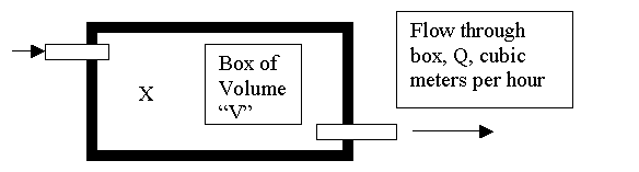
Start with an amount "X" (say in kilograms), in a volume "V"
(say in cubic meters). Then the
initial concentration is X/V. Call it C0. The flow of fluid through the box
is Q cubic meters per hour.
The concentration at any later time Ct is
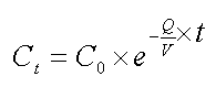
The Q/V term is the rate constant and it has units of inverse time, t-1.
Often the rate constant symbolized by a lower case "k."
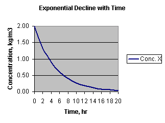
Here's a graph of that change in concentration with time:
You can see that calculations by clicking here.
From the graph you could see that the time for the concentration to drop from
2.00 to 1.00 is about 3.5 hours. You can also see that in the next 3.5 hours,
the concentration drops from 1.00 to 0.5, again half. That time, 3.5 hours in
this case, is called the "half-life" given the symbol t1/2.
Above, the Y axis is an arithmetic scale. Here it is on a log scale:
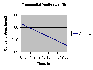
for a first order rate constant, there is a fixed relation between the rate
constant and the half life:
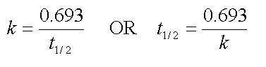
If you plotted the log of the concentration versus time and found a straight line, you could use the above relationships to determine "k."
For a one compartment model, the volume of distribution of a chemical is easy to calculate. Say you give a chemical that rapidly equilibrates through the body, methanol, would be a good example. Give the chemical i.p. and measure the concentration in the blood. Here's what you you would see.
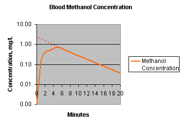 |
The solid orange line is the concentration of methanol as it moves away from the peritoneum and equilibrate throughout the body, about minute 6 this equilibration is complete and the decline after that is due to first order elimination of the chemical. The dashed line, extrapolates back to the concentration at time zero. The mass of methanol injected, divided by the extrapolated concentration at time zero (before any elimination takes place) yields the volume of distribution. |